Using the TimeSeriesAnalysis Package

Overview

This document aims to showcase how to use the TimeSeriesAnalysis package for the sample data sets included in the package.

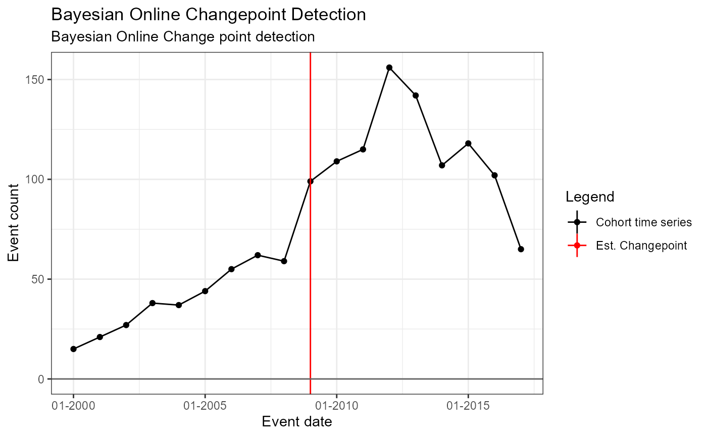
Data set 1: Changes in use of HCQ in RA patients over time

Background: RA guidelines recommend using Methotrexate as first line therapy ASAP from 2008, possibly ‘displacing’ hydroxychloroquine (HCQ).

Period: 2000 – 2018

outputFolder <- "E:/Timeseries/HCQ_In_RA_Example"
if (dir.exists(outputFolder)) {
  unlink(outputFolder, recursive = TRUE)
}
data(drugData)

# HCQ Use in RA Patients is cohortDefinitionId == 3
tsData <- drugData %>%
  filter(cohortDefinitionId == 3) %>%
  arrange(cohortStartDate) %>%
  select(cohortStartDate, subjectCount) %>%
  rename(
    eventDate = cohortStartDate,
    eventCount = subjectCount
  )

tsData

## # A tibble: 18 x 2
##    eventDate  eventCount
##    <date>          <dbl>
##  1 2000-01-01         15
##  2 2001-01-01         21
##  3 2002-01-01         27
##  4 2003-01-01         38
##  5 2004-01-01         37
##  6 2005-01-01         44
##  7 2006-01-01         55
##  8 2007-01-01         62
##  9 2008-01-01         59
## 10 2009-01-01         99
## 11 2010-01-01        109
## 12 2011-01-01        115
## 13 2012-01-01        156
## 14 2013-01-01        142
## 15 2014-01-01        107
## 16 2015-01-01        118
## 17 2016-01-01        102
## 18 2017-01-01         65

Creating the model arguments

The following sections will describe how to define the various model fitting arguments for several use cases.

Single Pre-specified change point – fixed (i.e. no estimated changepoint produced by model)

In this example, we’ll create the arguments used to fit a model that has no estimated change points and instead provides a single pre-specified change point for evaluation.

segArgs1 <- createSegmentedArgs(
  modelType = "linear",
  psi = lubridate::as_date("2001-01-01"),
  control = segmented::seg.control(
    it.max = 0,
    K = 1
  )
)

Single prespecified changepoint – not fixed (i.e. an estimated changepoint produced by model which may or may no coincide with pre-specified change point)

Now we’ll create the arguments used to fit a model that has 1 estimated change points and a single pre-specified change point for evaluation.

segArgs2 <- createSegmentedArgs(
  modelType = "linear",
  npsi = 1,
  fixed.psi = list(eventDate = lubridate::as_date("2001-01-01"))
)

No prespecified changepoint – an estimated changepoint produced by model

Now we’ll create the arguments used to fit a model with a single estimated change point

segArgs3 <- createSegmentedArgs(modelType = "linear")

Single prespecified changepoint – and multiple estimated changepoints produced by model

Now we’ll create the arguments used to fit a model with a single pre-specified changepoint and 2 estimated changepoints.

segArgs4 <- createSegmentedArgs(
  modelType = "linear",
  npsi = 2,
  fixed.psi = list(eventDate = lubridate::as_date("2001-01-01"))
)

Bayesian Online Change point detection

ocpArgs <- TimeSeriesAnalysis::createOcpArgs()

Fitting the models

Next we’ll provide some code for using the arguments and data above to fit the models.

# Create the full set of analyses
tsAnalysis1 <- createTsAnalysis(
  analysisId = 1,
  description = "Single fixed, pre-specified change point",
  tsArgs = segArgs1
)
tsAnalysis2 <- createTsAnalysis(
  analysisId = 2,
  description = "1 pre-specified, 1 estimated changepoint",
  tsArgs = segArgs2
)
tsAnalysis3 <- createTsAnalysis(
  analysisId = 3,
  description = "Single estimated changepoint",
  tsArgs = segArgs3
)
tsAnalysis4 <- createTsAnalysis(
  analysisId = 4,
  description = "1 pre-specified, 2 estimated changepoints",
  tsArgs = segArgs4
)
tsAnalysis5 <- createTsAnalysis(
  analysisId = 5,
  description = "Bayesian Online Change point detection",
  tsArgs = ocpArgs
)

tsAnalysisList <- list(tsAnalysis1, tsAnalysis2, tsAnalysis3, tsAnalysis4, tsAnalysis5)

# Run the analysis
runTsAnalyses(
  tsData = tsData,
  tsDataId = 1, # A unique identifier for the data set
  outputFolder = outputFolder,
  tsAnalysisList = tsAnalysisList
)

## Building time series models

## Analysis 1: Single fixed, pre-specified change point

## Analysis 2: 1 pre-specified, 1 estimated changepoint

## Analysis 3: Single estimated changepoint

## Analysis 4: 1 pre-specified, 2 estimated changepoints

## Analysis 5: Bayesian Online Change point detection

Inspecting the results

Next we can use the package to plot the original time series and the model estimated change points.

Single Pre-specified change point – fixed (i.e. no estimated changepoint produced by model)

m1 <- readRDS(file = file.path(outputFolder, "Analysis1/ts_d1.rds"))
TimeSeriesAnalysis::plotSegmented(m1$tsData, m1$model, plotSubtitle = tsAnalysisList[[1]]$description)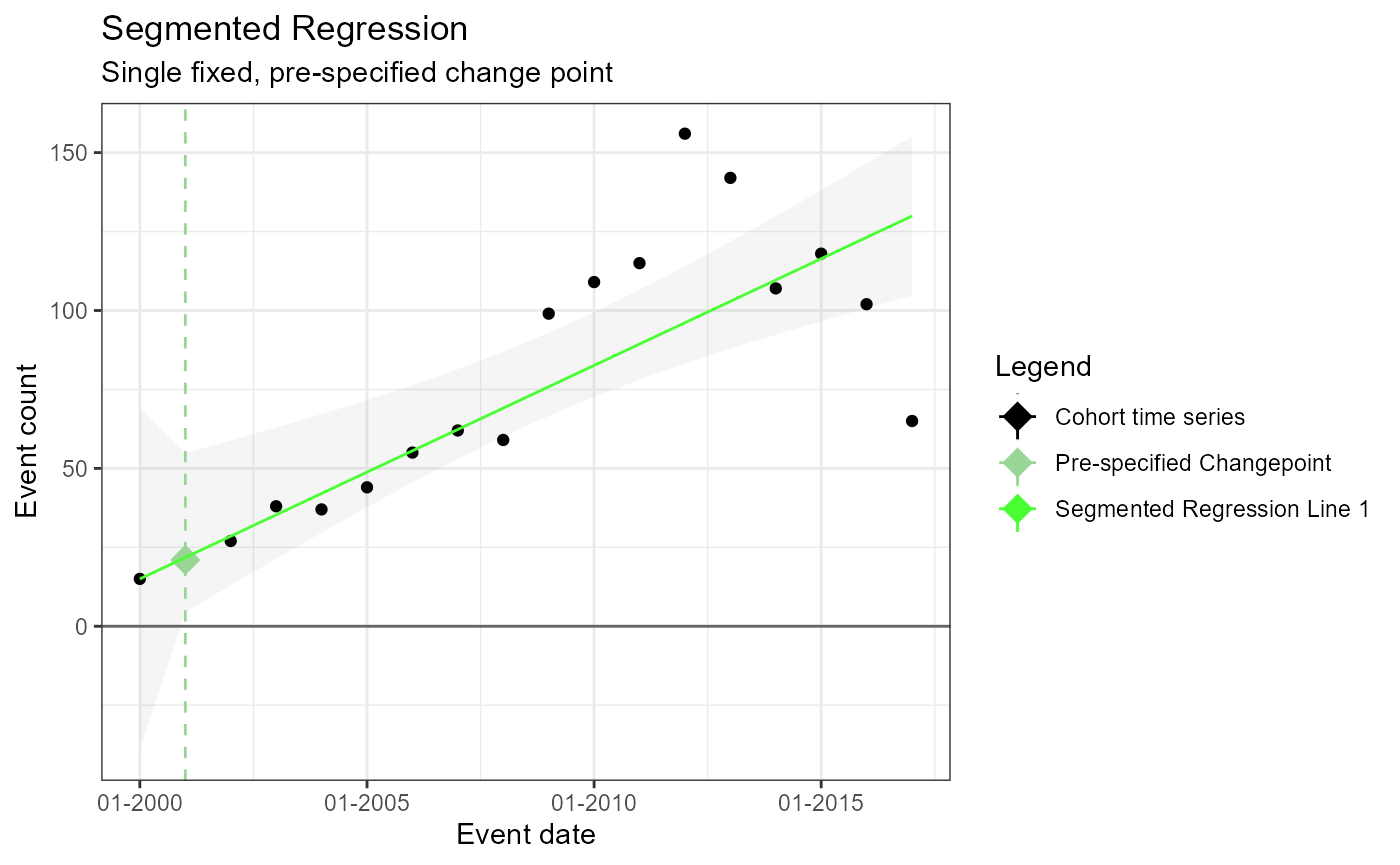

Single prespecified changepoint – not fixed (i.e. an estimated changepoint produced by model which may or may no coincide with pre-specified change point)

m2 <- readRDS(file = file.path(outputFolder, "Analysis2/ts_d1.rds"))
TimeSeriesAnalysis::plotSegmented(m2$tsData, m2$model, plotSubtitle = tsAnalysisList[[2]]$description)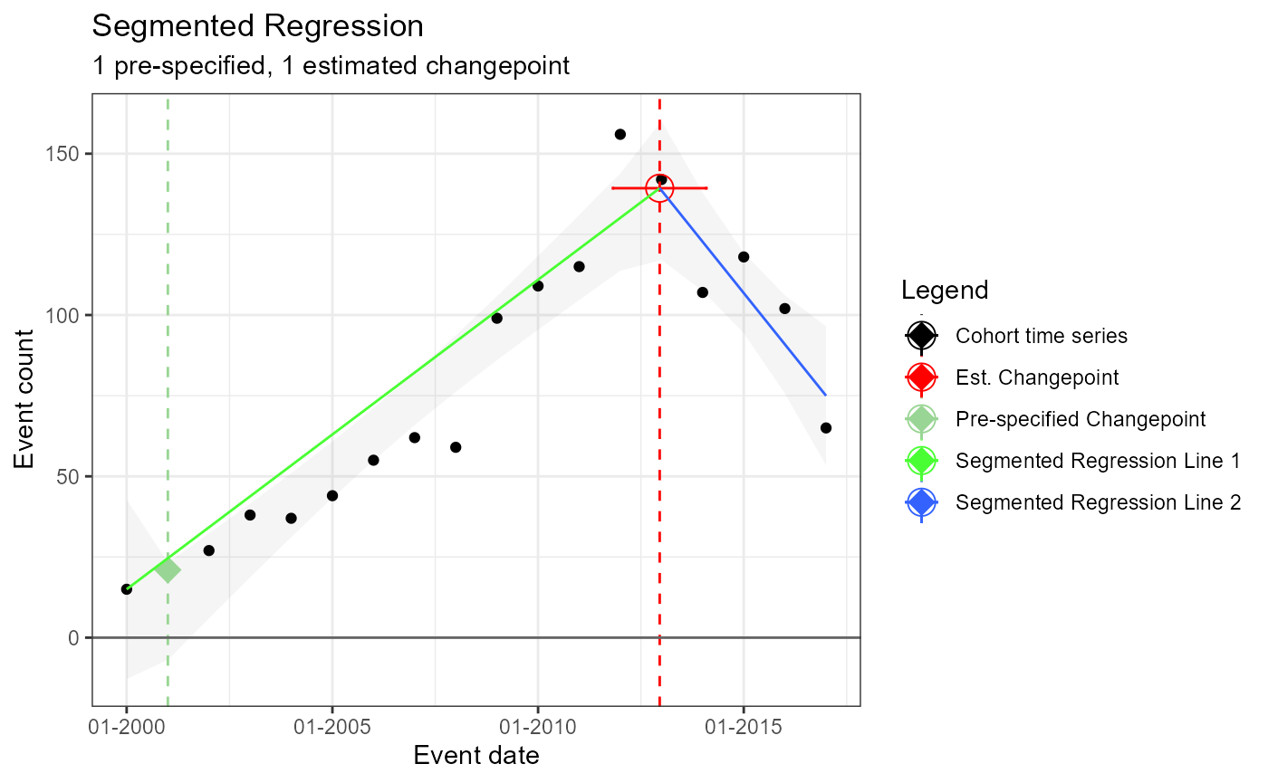

No prespecified changepoint – an estimated changepoint produced by model

m3 <- readRDS(file = file.path(outputFolder, "Analysis3/ts_d1.rds"))
TimeSeriesAnalysis::plotSegmented(m3$tsData, m3$model, plotSubtitle = tsAnalysisList[[3]]$description)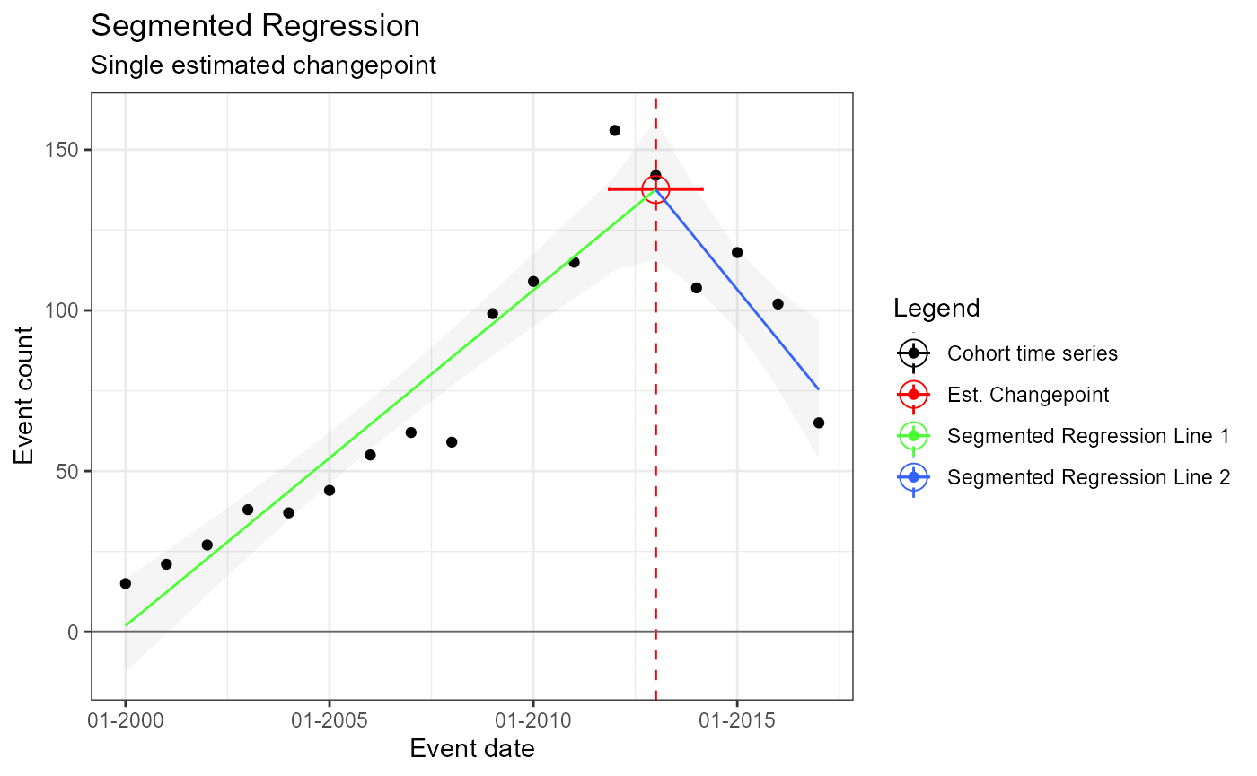

Single prespecified changepoint – and multiple estimated changepoints produced by model

m4 <- readRDS(file = file.path(outputFolder, "Analysis4/ts_d1.rds"))
TimeSeriesAnalysis::plotSegmented(m4$tsData, m4$model, plotSubtitle = tsAnalysisList[[4]]$description)

## Warning in matrix(newZ, nrow = nrow(newZ), ncol = length(psi.noti)): data
## length differs from size of matrix: [36 != 18 x 1]

## Warning in matrix(newZ, nrow = nrow(newZ), ncol = length(psi.noti)): data
## length differs from size of matrix: [36 != 18 x 1]

## Warning in matrix(newZ, nrow = nrow(newZ), ncol = length(psi.noti)): data
## length differs from size of matrix: [2 != 1 x 1]

## Warning in matrix(newZ, nrow = nrow(newZ), ncol = length(psi.noti)): data
## length differs from size of matrix: [2 != 1 x 1]

## Warning in matrix(newZ, nrow = nrow(newZ), ncol = length(psi.noti)): data
## length differs from size of matrix: [2 != 1 x 1]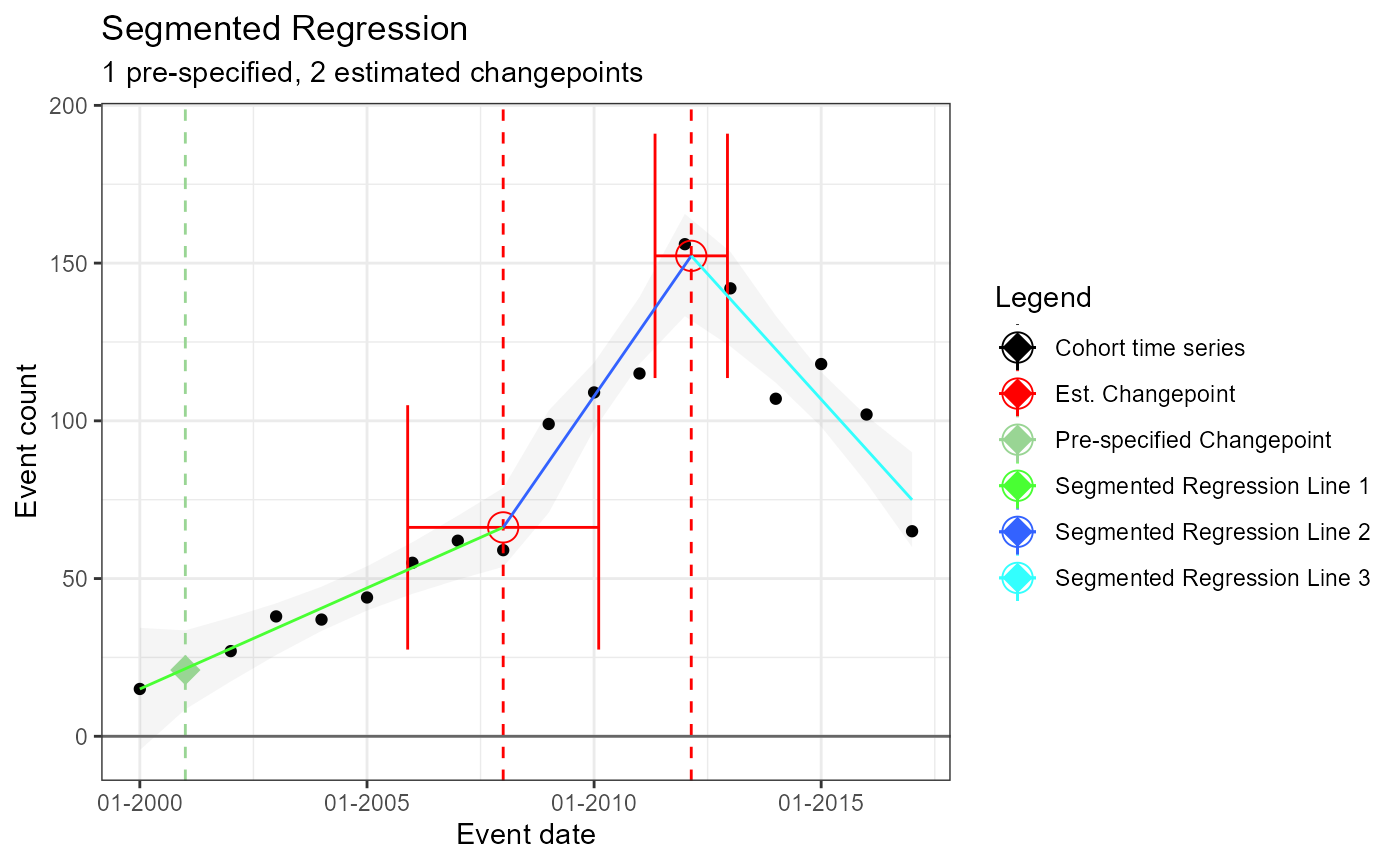

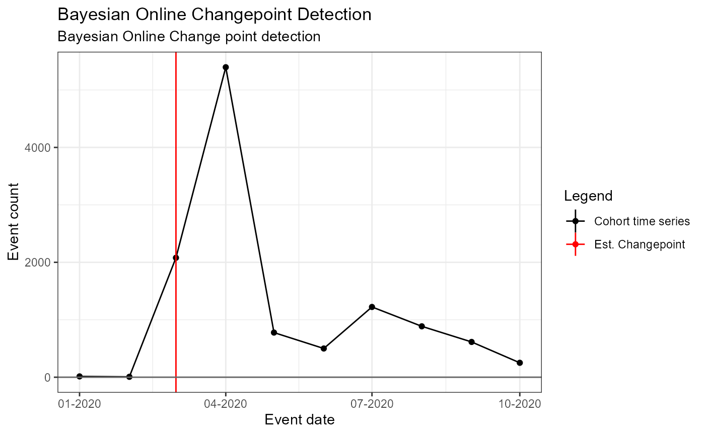
Bayesian Online Change point detection

m5 <- readRDS(file = file.path(outputFolder, "Analysis5/ts_d1.rds"))
TimeSeriesAnalysis::plotOcp(m5$tsData, m5$model, plotSubtitle = tsAnalysisList[[5]]$description)

Data Set 2: HCQ for Covid-19 in 2020

Background: - HCQ received emergency approval by FDA in March - Regulatory action followed in late April due to CV safety issues - Data: HCQ for Covid-19 treatment - Period: Jan – Oct 2020

outputFolder <- "E:/Timeseries/HCQ_In_COVID"
if (dir.exists(outputFolder)) {
  unlink(outputFolder, recursive = TRUE)
}

# HCQ for Covid-19 in 2020 is cohortDefinitionId == 1
tsData <- drugData %>%
  filter(cohortDefinitionId == 1) %>%
  arrange(cohortStartDate) %>%
  select(cohortStartDate, subjectCount) %>%
  rename(
    eventDate = cohortStartDate,
    eventCount = subjectCount
  )

tsData

## # A tibble: 10 x 2
##    eventDate  eventCount
##    <date>          <dbl>
##  1 2020-01-01         14
##  2 2020-02-01          7
##  3 2020-03-01       2079
##  4 2020-04-01       5396
##  5 2020-05-01        777
##  6 2020-06-01        500
##  7 2020-07-01       1223
##  8 2020-08-01        886
##  9 2020-09-01        614
## 10 2020-10-01        251

Single Pre-specified change point – fixed (i.e. no estimated changepoint produced by model)

segArgs1 <- createSegmentedArgs(
  modelType = "linear",
  psi = lubridate::as_date("2020-03-01"),
  control = segmented::seg.control(
    it.max = 0,
    K = 1
  )
)

Single prespecified changepoint – not fixed (i.e. an estimated changepoint produced by model which may or may no coincide with pre-specified change point)

segArgs2 <- createSegmentedArgs(
  modelType = "linear",
  npsi = 1,
  fixed.psi = list(eventDate = lubridate::as_date("2020-03-01"))
)

No prespecified changepoint – an estimated changepoint produced by model

Now we’ll create the arguments used to fit a model with a single estimated change point

segArgs3 <- createSegmentedArgs(modelType = "linear")

Single prespecified changepoint – and multiple estimated changepoints produced by model

Now we’ll create the arguments used to fit a model with a single pre-specified changepoint and 2 estimated changepoints.

segArgs4 <- createSegmentedArgs(
  modelType = "linear",
  npsi = 2,
  fixed.psi = list(eventDate = lubridate::as_date("2020-03-01"))
)

Fitting the models

Next we’ll provide some code for using the arguments and data above to fit the models.

# Create the full set of analyses
tsAnalysis1 <- createTsAnalysis(
  analysisId = 1,
  description = "Single fixed, pre-specified change point",
  tsArgs = segArgs1
)
tsAnalysis2 <- createTsAnalysis(
  analysisId = 2,
  description = "1 pre-specified, 1 estimated changepoint",
  tsArgs = segArgs2
)
tsAnalysis3 <- createTsAnalysis(
  analysisId = 3,
  description = "Single estimated changepoint",
  tsArgs = segArgs3
)
tsAnalysis4 <- createTsAnalysis(
  analysisId = 4,
  description = "1 pre-specified, 2 estimated changepoints",
  tsArgs = segArgs4
)
tsAnalysis5 <- createTsAnalysis(
  analysisId = 5,
  description = "Bayesian Online Change point detection",
  tsArgs = ocpArgs
)

tsAnalysisList <- list(tsAnalysis1, tsAnalysis2, tsAnalysis3, tsAnalysis4, tsAnalysis5)

# Run the analysis
runTsAnalyses(
  tsData = tsData,
  tsDataId = 2, # A unique identifier for the data set
  outputFolder = outputFolder,
  tsAnalysisList = tsAnalysisList
)

## Building time series models

## Analysis 1: Single fixed, pre-specified change point

## Analysis 2: 1 pre-specified, 1 estimated changepoint

## Warning encountered when fitting segmented model: No breakpoint estimated

## Analysis 3: Single estimated changepoint

## Analysis 4: 1 pre-specified, 2 estimated changepoints

## breakpoint estimate(s): 18353 18444

## Error encountered when fitting segmented model: at least one coef is NA: breakpoint(s) at the boundary? (possibly with many x-values replicated)

## Analysis 5: Bayesian Online Change point detection

Inspect the results

Single Pre-specified change point – fixed (i.e. no estimated changepoint produced by model)

m1 <- readRDS(file = file.path(outputFolder, "Analysis1/ts_d2.rds"))
TimeSeriesAnalysis::plotSegmented(m1$tsData, m1$model, plotSubtitle = tsAnalysisList[[1]]$description)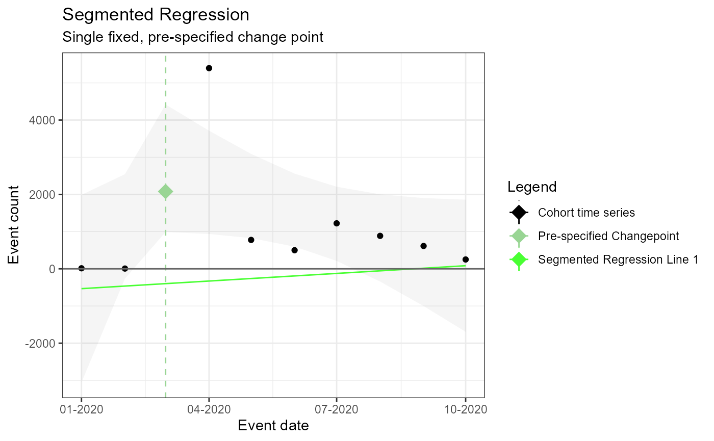

Single prespecified changepoint – not fixed (i.e. an estimated changepoint produced by model which may or may no coincide with pre-specified change point)

m2 <- readRDS(file = file.path(outputFolder, "Analysis2/ts_d2.rds"))
TimeSeriesAnalysis::plotSegmented(m2$tsData, m2$model, plotSubtitle = tsAnalysisList[[2]]$description)

## Error in tryCatch(withCallingHandlers({: 1 assertions failed:
##  * Variable '!is.null(model)': Must be TRUE.

No prespecified changepoint – an estimated changepoint produced by model

m3 <- readRDS(file = file.path(outputFolder, "Analysis3/ts_d2.rds"))
TimeSeriesAnalysis::plotSegmented(m3$tsData, m3$model, plotSubtitle = tsAnalysisList[[3]]$description)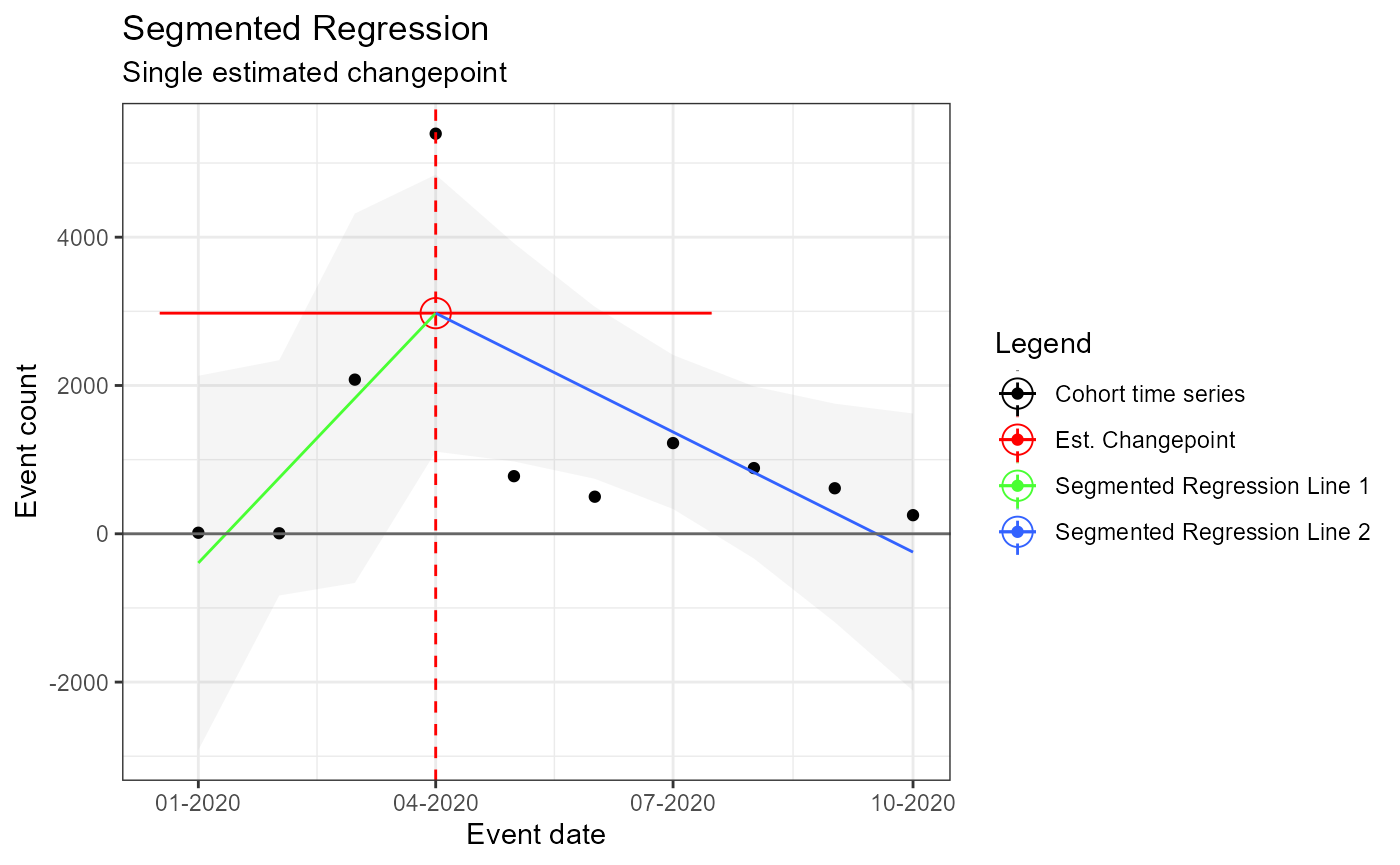

Single prespecified changepoint – and multiple estimated changepoints produced by model

m4 <- readRDS(file = file.path(outputFolder, "Analysis4/ts_d2.rds"))
TimeSeriesAnalysis::plotSegmented(m4$tsData, m4$model, plotSubtitle = tsAnalysisList[[4]]$description)

## Error in tryCatch(withCallingHandlers({: 1 assertions failed:
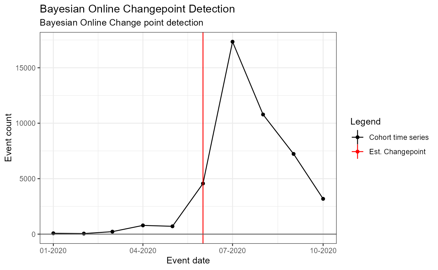
##  * Variable '!is.null(model)': Must be TRUE.

Bayesian Online Change point detection

m5 <- readRDS(file = file.path(outputFolder, "Analysis5/ts_d2.rds"))
TimeSeriesAnalysis::plotOcp(m5$tsData, m5$model, plotSubtitle = tsAnalysisList[[5]]$description)

Data Set 3: Dexamethasone for Covid-19 in 2020

Background: - RECOVERY RCT report 30% reduction in mortality in late June 2020 with dexamethasone (DXM) - Period: Jan – Oct 2020

outputFolder <- "E:/Timeseries/DEX_In_COVID"
if (dir.exists(outputFolder)) {
  unlink(outputFolder, recursive = TRUE)
}

# DEX for Covid-19 in 2020 is cohortDefinitionId == 2
tsData <- drugData %>%
  filter(cohortDefinitionId == 2) %>%
  arrange(cohortStartDate) %>%
  select(cohortStartDate, subjectCount) %>%
  rename(
    eventDate = cohortStartDate,
    eventCount = subjectCount
  )

tsData

## # A tibble: 10 x 2
##    eventDate  eventCount
##    <date>          <dbl>
##  1 2020-01-01         77
##  2 2020-02-01         51
##  3 2020-03-01        224
##  4 2020-04-01        787
##  5 2020-05-01        706
##  6 2020-06-01       4565
##  7 2020-07-01      17347
##  8 2020-08-01      10785
##  9 2020-09-01       7231
## 10 2020-10-01       3182

Single Pre-specified change point – fixed (i.e. no estimated changepoint produced by model)

segArgs1 <- createSegmentedArgs(
  modelType = "linear",
  psi = lubridate::as_date("2020-06-01"),
  control = segmented::seg.control(
    it.max = 0,
    K = 1
  )
)

Single prespecified changepoint – not fixed (i.e. an estimated changepoint produced by model which may or may no coincide with pre-specified change point)

segArgs2 <- createSegmentedArgs(
  modelType = "linear",
  npsi = 1,
  fixed.psi = list(eventDate = lubridate::as_date("2020-06-01"))
)

No prespecified changepoint – an estimated changepoint produced by model

Now we’ll create the arguments used to fit a model with a single estimated change point

segArgs3 <- createSegmentedArgs(modelType = "linear")

Single prespecified changepoint – and multiple estimated changepoints produced by model

Now we’ll create the arguments used to fit a model with a single pre-specified changepoint and 2 estimated changepoints.

segArgs4 <- createSegmentedArgs(
  modelType = "linear",
  npsi = 2,
  fixed.psi = list(eventDate = lubridate::as_date("2020-06-01"))
)

Fitting the models

Next we’ll provide some code for using the arguments and data above to fit the models.

# Create the full set of analyses
tsAnalysis1 <- createTsAnalysis(
  analysisId = 1,
  description = "Single fixed, pre-specified change point",
  tsArgs = segArgs1
)
tsAnalysis2 <- createTsAnalysis(
  analysisId = 2,
  description = "1 pre-specified, 1 estimated changepoint",
  tsArgs = segArgs2
)
tsAnalysis3 <- createTsAnalysis(
  analysisId = 3,
  description = "Single estimated changepoint",
  tsArgs = segArgs3
)
tsAnalysis4 <- createTsAnalysis(
  analysisId = 4,
  description = "1 pre-specified, 2 estimated changepoints",
  tsArgs = segArgs4
)
tsAnalysis5 <- createTsAnalysis(
  analysisId = 5,
  description = "Bayesian Online Change point detection",
  tsArgs = ocpArgs
)

tsAnalysisList <- list(tsAnalysis1, tsAnalysis2, tsAnalysis3, tsAnalysis4, tsAnalysis5)

# Run the analysis
runTsAnalyses(
  tsData = tsData,
  tsDataId = 3, # A unique identifier for the data set
  outputFolder = outputFolder,
  tsAnalysisList = tsAnalysisList
)

## Building time series models

## Analysis 1: Single fixed, pre-specified change point

## Analysis 2: 1 pre-specified, 1 estimated changepoint

## Warning encountered when fitting segmented model: No breakpoint estimated

## Analysis 3: Single estimated changepoint

## Analysis 4: 1 pre-specified, 2 estimated changepoints

## Warning encountered when fitting segmented model: No breakpoint estimated

## Analysis 5: Bayesian Online Change point detection

Inspect the results

Single Pre-specified change point – fixed (i.e. no estimated changepoint produced by model)

m1 <- readRDS(file = file.path(outputFolder, "Analysis1/ts_d3.rds"))
TimeSeriesAnalysis::plotSegmented(m1$tsData, m1$model, plotSubtitle = tsAnalysisList[[1]]$description)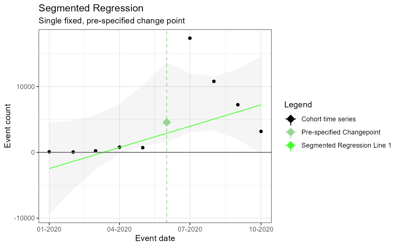

Single prespecified changepoint – not fixed (i.e. an estimated changepoint produced by model which may or may no coincide with pre-specified change point)

m2 <- readRDS(file = file.path(outputFolder, "Analysis2/ts_d3.rds"))
TimeSeriesAnalysis::plotSegmented(m2$tsData, m2$model, plotSubtitle = tsAnalysisList[[2]]$description)

## Error in tryCatch(withCallingHandlers({: 1 assertions failed:
##  * Variable '!is.null(model)': Must be TRUE.

No prespecified changepoint – an estimated changepoint produced by model

m3 <- readRDS(file = file.path(outputFolder, "Analysis3/ts_d3.rds"))
TimeSeriesAnalysis::plotSegmented(m3$tsData, m3$model, plotSubtitle = tsAnalysisList[[3]]$description)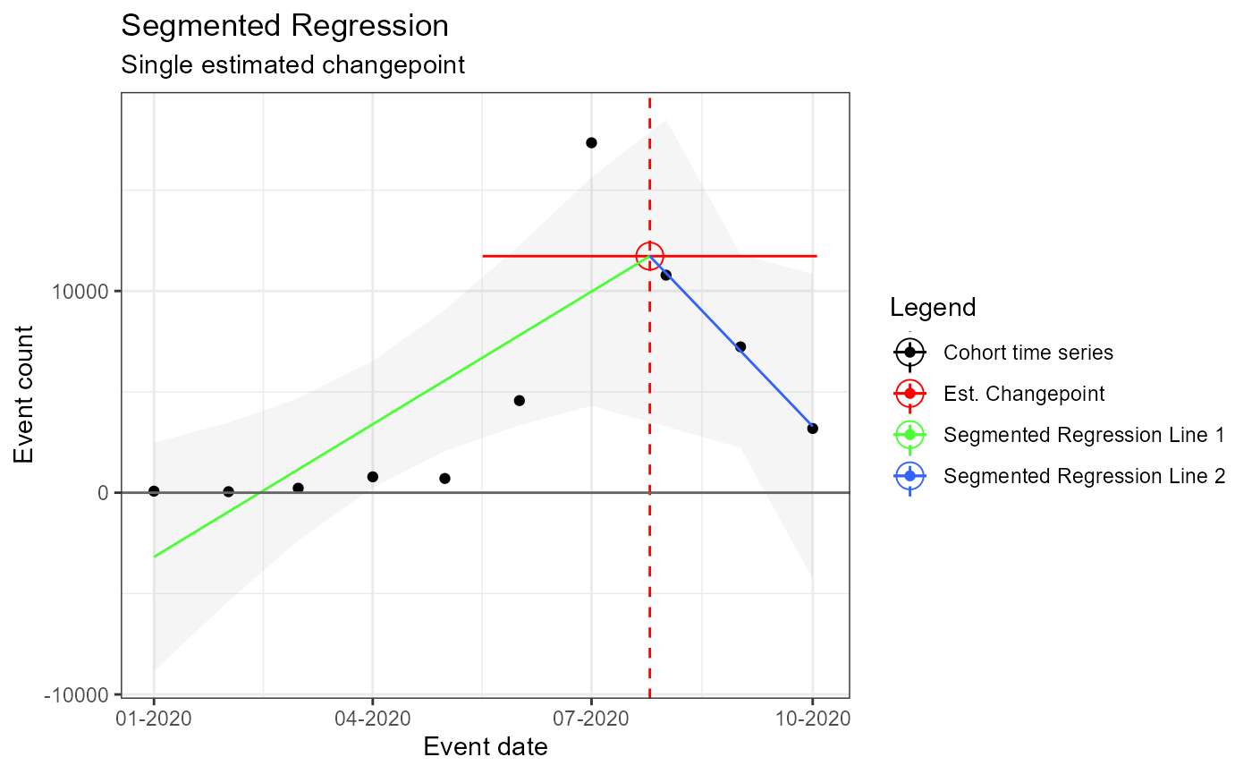

Single prespecified changepoint – and multiple estimated changepoints produced by model

m4 <- readRDS(file = file.path(outputFolder, "Analysis4/ts_d3.rds"))
TimeSeriesAnalysis::plotSegmented(m4$tsData, m4$model, plotSubtitle = tsAnalysisList[[4]]$description)

## Error in tryCatch(withCallingHandlers({: 1 assertions failed:
##  * Variable '!is.null(model)': Must be TRUE.

Bayesian Online Change point detection

m5 <- readRDS(file = file.path(outputFolder, "Analysis5/ts_d3.rds"))
TimeSeriesAnalysis::plotOcp(m5$tsData, m5$model, plotSubtitle = tsAnalysisList[[5]]$description)

Anthony G. Sena

2023-08-29

Overview

Data set 1: Changes in use of HCQ in RA patients over time

Creating the model arguments

Single Pre-specified change point – fixed (i.e. no estimated changepoint produced by model)

Single prespecified changepoint – not fixed (i.e. an estimated changepoint produced by model which may or may no coincide with pre-specified change point)

No prespecified changepoint – an estimated changepoint produced by model

Single prespecified changepoint – and multiple estimated changepoints produced by model

Bayesian Online Change point detection

Fitting the models

Inspecting the results

Single Pre-specified change point – fixed (i.e. no estimated changepoint produced by model)

Single prespecified changepoint – not fixed (i.e. an estimated changepoint produced by model which may or may no coincide with pre-specified change point)

No prespecified changepoint – an estimated changepoint produced by model

Single prespecified changepoint – and multiple estimated changepoints produced by model

Bayesian Online Change point detection

Data Set 2: HCQ for Covid-19 in 2020

Single Pre-specified change point – fixed (i.e. no estimated changepoint produced by model)

Single prespecified changepoint – not fixed (i.e. an estimated changepoint produced by model which may or may no coincide with pre-specified change point)

No prespecified changepoint – an estimated changepoint produced by model

Single prespecified changepoint – and multiple estimated changepoints produced by model

Fitting the models

Inspect the results

Single Pre-specified change point – fixed (i.e. no estimated changepoint produced by model)

Single prespecified changepoint – not fixed (i.e. an estimated changepoint produced by model which may or may no coincide with pre-specified change point)

No prespecified changepoint – an estimated changepoint produced by model

Single prespecified changepoint – and multiple estimated changepoints produced by model

Bayesian Online Change point detection

Data Set 3: Dexamethasone for Covid-19 in 2020

Single Pre-specified change point – fixed (i.e. no estimated changepoint produced by model)

Single prespecified changepoint – not fixed (i.e. an estimated changepoint produced by model which may or may no coincide with pre-specified change point)

No prespecified changepoint – an estimated changepoint produced by model

Single prespecified changepoint – and multiple estimated changepoints produced by model

Fitting the models

Inspect the results

Single Pre-specified change point – fixed (i.e. no estimated changepoint produced by model)

Single prespecified changepoint – not fixed (i.e. an estimated changepoint produced by model which may or may no coincide with pre-specified change point)

No prespecified changepoint – an estimated changepoint produced by model

Single prespecified changepoint – and multiple estimated changepoints produced by model

Bayesian Online Change point detection